The Overton Field

Abstract

This paper proposes a field-theoretic model of electoral politics in which the classical Overton window is replaced by an Overton field. The Overton field is a bounded region of political state-space whose geometry is shaped by parties, institutions, media, events, and electoral rules. Citizens are modeled as trajectories within this field, while parties are modeled as attractor poles generating basins of electoral capture. Election day is represented as a portal map from continuous political state-space to a finite set of admissible ballot outputs. In two-party systems, this portal map compresses a high-dimensional distribution of voter states into binary institutional form. The model explains how political complexity can persist at the level of belief while being reduced to two-pole capture at the level of electoral power. It also shows how parties do not merely compete inside the Overton window, but participate in constructing and deforming the field through which political states become votes.

1. Introduction

The usual account of the Overton window describes a range of policy ideas that politicians can support without losing public legitimacy. In that account, ideas inside the window are politically viable; ideas outside the window may exist, but politicians risk popular support by adopting them. The standard formulation is useful, but it is too static for modeling electoral systems. It describes a boundary around political possibility, but not the dynamics by which citizens move, parties attract, institutions compress, and votes emerge.

This paper replaces the window with a field. The Overton field is the region of political state-space that remains coupled to viable institutional outputs. A state inside the field can be processed by parties, media, electoral rules, public narratives, and administrative machinery. A state outside the field may be privately held or socially visible, but it has weak conversion into institutional power unless the field itself changes.

The model treats citizens as state-bearing agents moving through a political field. Their movement is shaped by personal conditions, information flows, social incentives, identity, events, and party attraction. Parties are treated not merely as alternatives on a ballot, but as field-generating poles. Election day is treated as a portal event: an institutional interface that converts continuous political states into a finite set of ballot outputs.

The central argument is that a two-party system creates two-pole capture. Citizens may occupy complex and internally mixed positions, but the voting mechanism does not accept a full political state. It accepts a discrete output. In a two-party system, this output is usually one party, the other party, or non-capture through abstention, invalidation, or refusal. Political complexity persists in the population, but the electoral portal compresses it into a low-dimensional institutional result.

2. Political state-space

Let \(\Omega_t \subset \mathbb{R}^n\) denote political state-space at time \(t\). A point \(x \in \Omega_t\) represents a possible political state. The coordinates of \(x\) need not correspond only to explicit policy positions. They may encode economic pressure, cultural orientation, institutional trust, perceived threat, class position, party identification, media exposure, symbolic attachment, local belonging, tactical expectation, and other politically relevant variables.

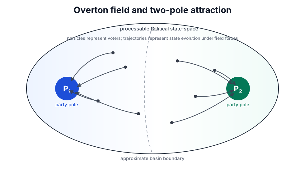
For each citizen \(i\), \(x_i(t)\) denotes that citizen’s political state at time \(t\). The population is represented by a measure \(\mu_t\) over \(\Omega_t\), where \(\mu_t(R)\) gives the mass of citizens occupying a region \(R \subseteq \Omega_t\). Public opinion is therefore not a single scalar quantity. It is a moving distribution over a high-dimensional field.

The classical Overton window can be represented as a projection of this field. If \(\pi : \Omega_t \to \mathbb{R}\) is a projection onto a simplified ideological axis, then the window is approximately an interval \(W_t = \pi(\Omega_t) \subset \mathbb{R}\), or a subinterval selected by a viability criterion. This projection can be useful for exposition, but it discards most of the geometry relevant to elections.

A voter can be economically redistributive, culturally conservative, anti-incumbent, locally loyal, institutionally distrustful, and tactically pragmatic at the same time. Such a state cannot be represented adequately by a single point on a left-right line. The field \(\Omega_t\), not the projected window \(W_t\), is therefore the primary object.

3. Voter motion

Voter motion through the field is modeled by a state-update equation. Let \(I_i(t)\) denote the informational environment encountered by citizen \(i\), including media, personal experience, conversation, polling, campaign messages, leader performances, prices, scandals, events, and institutional signals. Let \(E_t\) denote the broader environment of institutions, electoral rules, economic conditions, media structure, and collective events.

The function \(F_i\) is not assumed to be fully rational, homogeneous, or stable across all citizens. It is a compact representation of how political states update under influence. Some components of \(F_i\) may be deliberative, while others may be habitual, affective, social, or identity-based. The model requires only that incoming conditions can alter future political state.

In continuous time, the same idea can be written as a trajectory equation:

where \(\epsilon_i(t)\) captures shocks, idiosyncrasy, measurement error, and unmodeled influence. This term is not a claim that voter behavior is random. It acknowledges that no low-dimensional model will capture every causal input in a political life.

4. Party poles and attraction fields

Let \(P_1\) and \(P_2\) denote two dominant parties or blocs. Each party occupies a time-dependent position in political state-space:

Each party also generates an attraction field \(A_j(x,t)\), describing the directional pull exerted by party \(j\) on a citizen located at state \(x\) at time \(t\). The attraction field is produced by campaign strategy, institutional reputation, candidate selection, donor networks, media alignment, symbolic identity, policy offers, coalition memory, and negative polarization.

A general motion equation incorporating party attraction is:

The coefficients \(\alpha_{ij}(t)\) represent citizen-specific susceptibility to the attraction field of party \(j\). These coefficients may depend on identity, habit, social network, media diet, class position, perceived stakes, or prior allegiance. The field may include both attraction and repulsion. In highly polarized systems, a citizen may move toward one pole not because of positive affinity, but because of stronger repulsion from the other pole.

Parties therefore act as more than ballot labels. They shape the geometry of political motion. They pull some regions of state-space toward themselves, repel others, and compete to define which features of the environment become electorally salient. Their strategic objective is not merely to state positions, but to shape the routes by which citizens move through the field before reaching the ballot interface.

5. The Overton field

The Overton field is defined as the politically processable region of state-space:

This definition changes the emphasis of the Overton concept. The key issue is not simply whether a view can be spoken. The key issue is whether a political state can be processed into power. A view can be spoken frequently yet remain electorally inert. Another view can be poorly articulated but strongly coupled to institutional capture if a party, media system, or social movement links it to a viable ballot output.

The Overton field evolves over time. A compact field-update equation is:

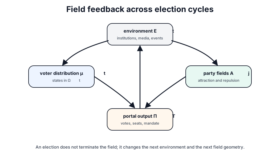
where \(S_t\) represents shocks such as wars, economic crises, scandals, court rulings, pandemics, assassinations, technological changes, or viral symbolic events. The field is endogenous. Parties compete within it, but they also deform it. Citizens move through it, but aggregate movement changes it. Institutions regulate it, but institutional outputs are themselves produced through prior field states.

6. The electoral portal

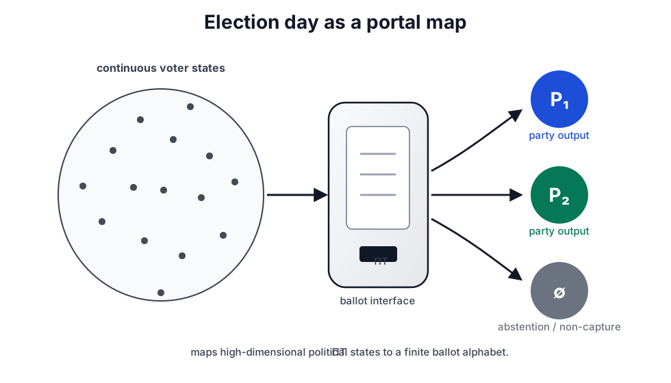
Election day is modeled as a portal event. At election time \(T\), each citizen’s continuous political state is passed through an institutional map:

where \(\mathcal{B}\) is the set of admissible ballot outputs. In a two-party system with abstention or failed capture,

where \(\varnothing\) represents abstention, invalidation, refusal, or non-capture. In a strict binary model that ignores abstention, \(\mathcal{B}=\{P_1,P_2\}\).

The vote is therefore:

This is the central compression event. A citizen may hold a complex, mixed, unstable, or non-party-aligned political state. The electoral interface does not accept the full vector. It accepts a ballot token. The portal transforms political complexity into institutional simplicity.

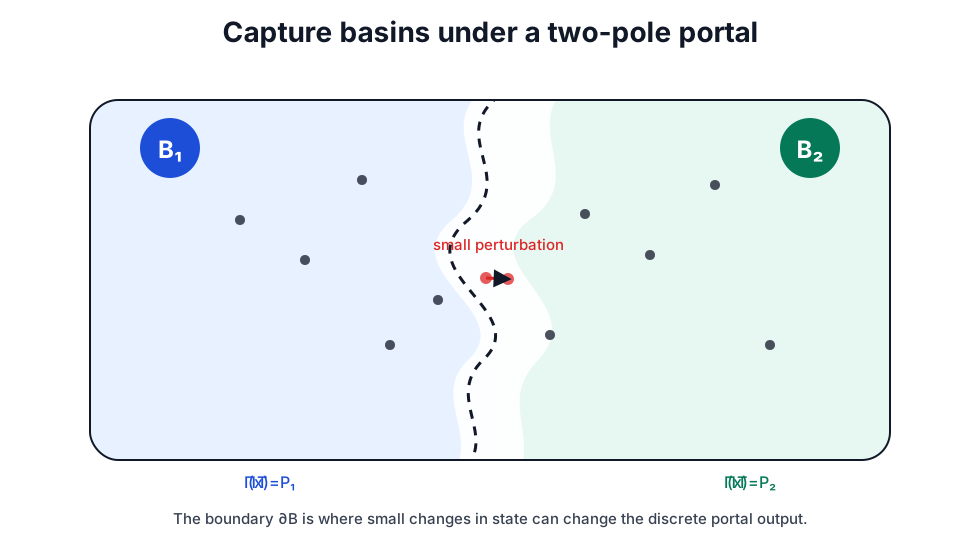
Define the capture basin of party \(P_j\) at time \(T\) as:

The non-capture basin is:

At the portal, the field is partitioned into regions that map to different outputs:

with overlaps of measure zero in the idealized case. The political meaning of a voter’s state at election time is determined by which basin contains it.

7. Binary compression theorem

The proposition does not claim that citizens are binary. It claims that the portal reports them as binary. The underlying distribution can remain high-dimensional, conflicted, and heterogeneous while the institutional output remains low-dimensional.

With abstention included, the portal alphabet becomes \(\{P_1,P_2,\varnothing\}\). The compression remains severe, but it is ternary rather than strictly binary. This distinction matters because parties may win by moving citizens into their own basin, by moving opponents into non-capture, or by preventing their own weak supporters from drifting into non-capture.

8. Field deformation and control

A party controls the field when it can influence voter motion, basin geometry, or the portal map. These are analytically distinct forms of power. Voter motion concerns how citizens move before the election. Basin geometry concerns which regions map to which party. The portal map concerns the institutional rule by which political states become ballot outputs.

Field control can therefore be represented through three interventions:

1. altering the informational environment \(I_i(t)\), thereby changing voter trajectories;
2. altering attraction fields \(A_j(x,t)\), thereby changing the geometry of pull and repulsion;
3. altering the portal \(\Pi_T\), thereby changing how states are converted into institutional outputs.

The first intervention includes messaging, agenda-setting, media amplification, scandal emphasis, and narrative framing. The second includes coalition strategy, candidate selection, symbolic repositioning, and negative polarization. The third includes electoral law, ballot access, districting, thresholds, voting technology, registration rules, and strategic voting incentives.

This framework explains why political struggle often concentrates near basin boundaries. Moving a citizen deep inside the opposing basin may be costly. Moving a citizen near \(\partial B\) may be decisive. A campaign can therefore produce large electoral effects without changing the entire distribution \(\mu_T\). It may only need to perturb enough boundary-adjacent mass, reshape the boundary, or change turnout probabilities inside weakly captured regions.

9. Nonlinear and strange-attractor-like dynamics

The model permits strange-attractor-like behavior without requiring the stronger claim that an empirical party system is formally a strange attractor. The weaker claim is sufficient: electoral fields may be bounded, nonlinear, and perturbation-sensitive. Boundedness comes from the processable field and the finite portal alphabet. Nonlinearity comes from the fact that political effects need not be proportional to the size of their causes. Perturbation sensitivity appears near basin boundaries, where small changes in state can alter the portal output.

If \(x\) lies near \(\partial B_1(T)\), then a small perturbation \(\delta x\) may change the output:

A scandal, price shock, viral phrase, leader error, court ruling, or local event can therefore have disproportionate effects when it reaches boundary-sensitive regions of the field. This does not imply that all politics is chaotic. It implies that the system can be locally unstable while remaining globally structured by dominant poles and institutional rules.

The field is also path-dependent. A party’s earlier positioning affects later susceptibility. A coalition built in one cycle alters the next field. A prior scandal changes the meaning of a later accusation. A voting rule that once looked neutral can produce durable expectations about viability. The system therefore has memory, and that memory affects both trajectories and capture basins.

10. Multi-party extension

The model generalizes to \(k\) parties. The portal map becomes:

The field is partitioned into \(k\) party basins plus non-capture:

In proportional systems, the portal may preserve more information from the underlying distribution because more outputs can produce representation. In plurality or winner-take-all systems, the effective portal may contain fewer viable outputs than the formal ballot. A voter may see many names on the ballot while perceiving only two viable destinations for political power.

This distinction separates formal party count from effective capture count. A system may have many legal parties but still behave as a two-pole field if media attention, strategic voting, coalition logic, ballot access, or electoral rules compress viable outcomes. Conversely, a system may contain two major parties but include internal factions that behave as sub-basins inside each major pole.

11. Empirical interpretation

The model can be interpreted empirically by estimating a political state-space from survey data, issue positions, turnout history, demographic variables, media exposure, institutional trust, and affective polarization measures. Dimensionality-reduction methods can produce an approximate field, while classification methods can estimate the portal map from state vectors to observed vote outputs.

The key empirical objects are the distribution \(\mu_t\), the capture basins \(B_j(T)\), the basin boundary \(\partial B\), and the sensitivity of that boundary to perturbations. A campaign effect can be modeled as a deformation of either the distribution or the portal-induced partition. A persuasion campaign moves mass through the field. A turnout campaign changes the measure assigned to non-capture. A framing campaign changes the geometry of capture by changing which dimensions become decisive.

Useful observables include estimated distance from basin boundaries, rates of cross-pressure within state-space, local turnout elasticity, local persuasion elasticity, and the effective number of portal outputs. The model predicts that high-dimensional political disagreement may coexist with stable two-party outcomes when the portal is strongly compressive.

12. Implications

The model reframes political agency. Citizens are not passive particles in a deterministic field, but neither are they isolated rational choosers selecting from neutral options. They are state-bearing agents embedded in informational, social, and institutional fields. Their political motion depends on both internal disposition and external geometry.

The model also reframes campaigns. A campaign is not merely a sequence of persuasive statements. It is an attempt to alter voter trajectories, reshape basin boundaries, change turnout probabilities, and modify the portal conditions under which states become votes. This is why campaigns frequently concentrate on salience rather than argument. Changing which dimension matters can be more effective than changing a voter’s entire ideology.

The model reframes party power. Parties do not simply compete inside a pre-existing Overton window. They participate in constructing the field. They decide which measurements become salient, which identities are activated, which grievances are routed toward which pole, which fears are amplified, which compromises are made costly, and which ballot outputs appear viable.

Finally, the model reframes the vote. A vote is not the full expression of a citizen’s political state. It is the admissible output accepted by the portal. The ballot is therefore a compression device. It converts a high-dimensional political life into a low-dimensional institutional signal.

13. Limitations

This paper provides a formal model, not a completed empirical identification strategy. The state-space \(\Omega_t\), the voter distribution \(\mu_t\), the attraction fields \(A_j\), and the portal map \(\Pi_T\) must be estimated or operationalized differently across electoral systems. The model is therefore a framework for analysis rather than a ready-made measurement instrument.

The model also abstracts from many institutional details. Electoral colleges, bicameral systems, primaries, coalition formation, compulsory voting, ranked-choice systems, party lists, thresholds, and district boundaries can each change the portal map. These details should be treated as modifications of \(\Pi_T\), not as peripheral complications.

The strange-attractor language remains metaphorical unless a specific dynamical system is specified and shown to satisfy the relevant formal conditions. The core claim of the paper does not depend on that stronger result. It depends on field motion, basin capture, and portal compression.

14. Conclusion

This paper has proposed the Overton field as a replacement for the static window metaphor. The political field is a region of processable state-space through which citizens move under the influence of information, social pressure, institutional structure, events, and party attraction. Parties act as poles that shape the geometry of movement and define basins of electoral capture. Election day is a portal event that maps continuous political states to finite ballot outputs.

In a two-party system, this creates binary compression. The population can contain a complex distribution of beliefs, values, attachments, and grievances, yet the institutional mechanism reports that distribution as a contest between two dominant poles. Political complexity is not absent. It is compressed.

The Overton field therefore names the operating space in which political possibility becomes institutional power. It is not simply the range of what may be said. It is the field in which voters move, parties attract, boundaries shift, perturbations matter, and votes emerge as compressed signals from a much larger political state-space.

References

Bochsler, D. (2022). “Duverger and the territory: explaining deviations from the two-party system in plurality elections.” Journal of Elections, Public Opinion and Parties. https://www.tandfonline.com/doi/full/10.1080/17457289.2019.1658195
Daza, A., Wagemakers, A., & Sanjuán, M. A. F. (2022). “Classifying basins of attraction using the basin entropy.” Communications in Nonlinear Science and Numerical Simulation. Preprint: https://arxiv.org/abs/2201.08083
Duverger, M. (1964). Political Parties: Their Organization and Activity in the Modern State. London: Methuen.
Laakso, M., & Taagepera, R. (1979). “Effective number of parties: A measure with application to West Europe.” Comparative Political Studies, 12(1), 3–27.
Lehman, J. G. (2010). “An Introduction to the Overton Window of Political Possibility.” Mackinac Center for Public Policy. https://www.mackinac.org/12481
Mackinac Center for Public Policy. “The Overton Window.” https://www.mackinac.org/OvertonWindow
Riker, W. H. (1982). “The Two-party System and Duverger’s Law: An Essay on the History of Political Science.” American Political Science Review, 76(4), 753–766.